Friday, May 23, 2014


Tuesday, May 13, 2014
Mon. Week 12, May 12: Applications of Magnetic Force
On this day we set out to learn how the properties of magnatism that we learned from the previous class could be used in practical situations. One of these applications is the motor, a device that converts electrical energy into rotational motion. The motor is the heart of all automation and motion in electric devices.
The first exercise we performed was energizing a small motor and seeing how changing the magnetic field through it affects its motion.

After developing an intuitive understanding of how the orientation of the magnetic field affects the torque on the coil windings, we then set out to make our own motors from just wire with a current passing through it and a magnet.

After taking some time to make various adjustments, the simple motor proved to be operational and the exercise was a success.

The first exercise we performed was energizing a small motor and seeing how changing the magnetic field through it affects its motion.
After developing an intuitive understanding of how the orientation of the magnetic field affects the torque on the coil windings, we then set out to make our own motors from just wire with a current passing through it and a magnet.
After taking some time to make various adjustments, the simple motor proved to be operational and the exercise was a success.
Monday, May 12, 2014
Wed. Week 11, May 7: Intro to Magnetism
Magnetism was today's topic of conversation. Permanent magnets are made up of elements that contain a large number of electrons alone in their orbitals. The unpaired electrons create a field that is similar to the electric field created by a charge. This field is known as the magnetic field and has many important properties that relate to electric current and force.
The first exercise of the day was drawing up our predictions of the magnetic field for a bar magnet. The field lines extend from the north to south pole of the magnet and the magnetic flux through any closed surface is always zero.

We eventually came to the topic of how magnetic fields interact with moving charges. Since a moving charge exerts a magnetic field, it will interact with any external magnetic field, which will in turn apply a force on that moving charge. The resulting force is referred to as magnetic force and acts in the direction that is perpendicular to the directions of the charge's velocity and the external magnetic field. With this in mind, we deduced that a charge traveling at constant velocity with travel in a circular path within a uniform magnetic field.

After deriving several equations for magnetic force, we performed an experiment to find the value of the magnetic field for a bar of specific length, with a specific current running through it, moving at a specific acceleration.

The first exercise of the day was drawing up our predictions of the magnetic field for a bar magnet. The field lines extend from the north to south pole of the magnet and the magnetic flux through any closed surface is always zero.
We eventually came to the topic of how magnetic fields interact with moving charges. Since a moving charge exerts a magnetic field, it will interact with any external magnetic field, which will in turn apply a force on that moving charge. The resulting force is referred to as magnetic force and acts in the direction that is perpendicular to the directions of the charge's velocity and the external magnetic field. With this in mind, we deduced that a charge traveling at constant velocity with travel in a circular path within a uniform magnetic field.
After deriving several equations for magnetic force, we performed an experiment to find the value of the magnetic field for a bar of specific length, with a specific current running through it, moving at a specific acceleration.
Mon. Week 11, May 5: Intro to Electronics
The subject of this day's lecture and lab was that of electronics, more specifically, the diode and the transistor. The diode is a component made up of two layers of a semiconductor material that has been doped with elements that give one of the layers a significant amount of free electrons and the other layer a significant amount of electron holes. When these two layers are brought into contact, the free electrons and holes combine and create what is know as the depletion region. If voltage is applied in one direction, the region shrinks and the diode acts as a conductor, but when voltage is applied in the reverse direction, the region grows and becomes and insulator, making the diode a one-way street for current. The transistor is essentially two diodes place back to back and has the ability to act as a switch.
For the first exercise of the day, we were tasked with created a circuit that displayed the voltage amplifying abilities of the transistor. When a signal was applied to the input of the circuit, that signal would be significantly larger in magnitude at the output.

With the oscilloscope connected to the input and output of our circuit, we were able to verify that the signal had indeed be amplified.

We also noticed that the output signal would get cutoff if we applied too much voltage on the input signal. We learned that this was due to the transistor being driven into saturation from the large amounts of voltage being applied to the base.

The transistor is a three lead component. Each lead corresponds to parts of the transistor known as the emitter, collector and base.

For the final portion of the day, we were introduced to the op-amp and the concept of integrated circuitry. An integrated circuit is an entire circuit that is boxed as an individual component. The op-amp is an integrated circuit that can act as a voltage comparator. By using the properties of feedback, the op-amp can be used as a signal amplifier much like the circuit that was previously built.

The amplifier circuit was built and tested with the output from a device that is capable of outputting sound to a speaker jack such as a phone. The low voltage signal was passed through the circuit and sent to a speaker, where the low voltage signal had gained enough voltage to be loud enough for everyone the hear.

For the first exercise of the day, we were tasked with created a circuit that displayed the voltage amplifying abilities of the transistor. When a signal was applied to the input of the circuit, that signal would be significantly larger in magnitude at the output.
With the oscilloscope connected to the input and output of our circuit, we were able to verify that the signal had indeed be amplified.
We also noticed that the output signal would get cutoff if we applied too much voltage on the input signal. We learned that this was due to the transistor being driven into saturation from the large amounts of voltage being applied to the base.
For the final portion of the day, we were introduced to the op-amp and the concept of integrated circuitry. An integrated circuit is an entire circuit that is boxed as an individual component. The op-amp is an integrated circuit that can act as a voltage comparator. By using the properties of feedback, the op-amp can be used as a signal amplifier much like the circuit that was previously built.
The amplifier circuit was built and tested with the output from a device that is capable of outputting sound to a speaker jack such as a phone. The low voltage signal was passed through the circuit and sent to a speaker, where the low voltage signal had gained enough voltage to be loud enough for everyone the hear.
Friday, May 2, 2014
Wed. Week 10, April 30: The Oscilloscope
Today we were introduced to the oscilloscope. An oscilloscope is a measurement device used to show how a voltage through a particular circuit changes with time. Oscilloscopes a particularly useful in trouble shooting AC circuits.
We started the day off with an kinematics exercise that had us find the distance an electron will travel between a set of charged plates. This exercise led to a live demonstration of an electron beam whose position was being aimed with external voltages on a series of plates that the beam traveled through. The purpose of this demonstration was to show the class the inner mechanics of the oscilloscopes display screen.

The next exercise of the day consisted of connecting a function generator to a speaker and having the generator output frequencies in the audible range. A function generator is a device that is capable of outputting an AC voltage at specific frequencies and wave shape. We learned that the frequency of the signal controls the pitch of the sound from the speaker, and the magnitude of the output voltage controlled the loudness.

The next exercise was measuring the voltage of a battery with the oscilloscope using a tap key in series with the battery. With the oscilloscope set to DC coupling, and appropriate values for volts/div and time/div set, we were able to measure the voltage of the battery at around 1.2 volts.
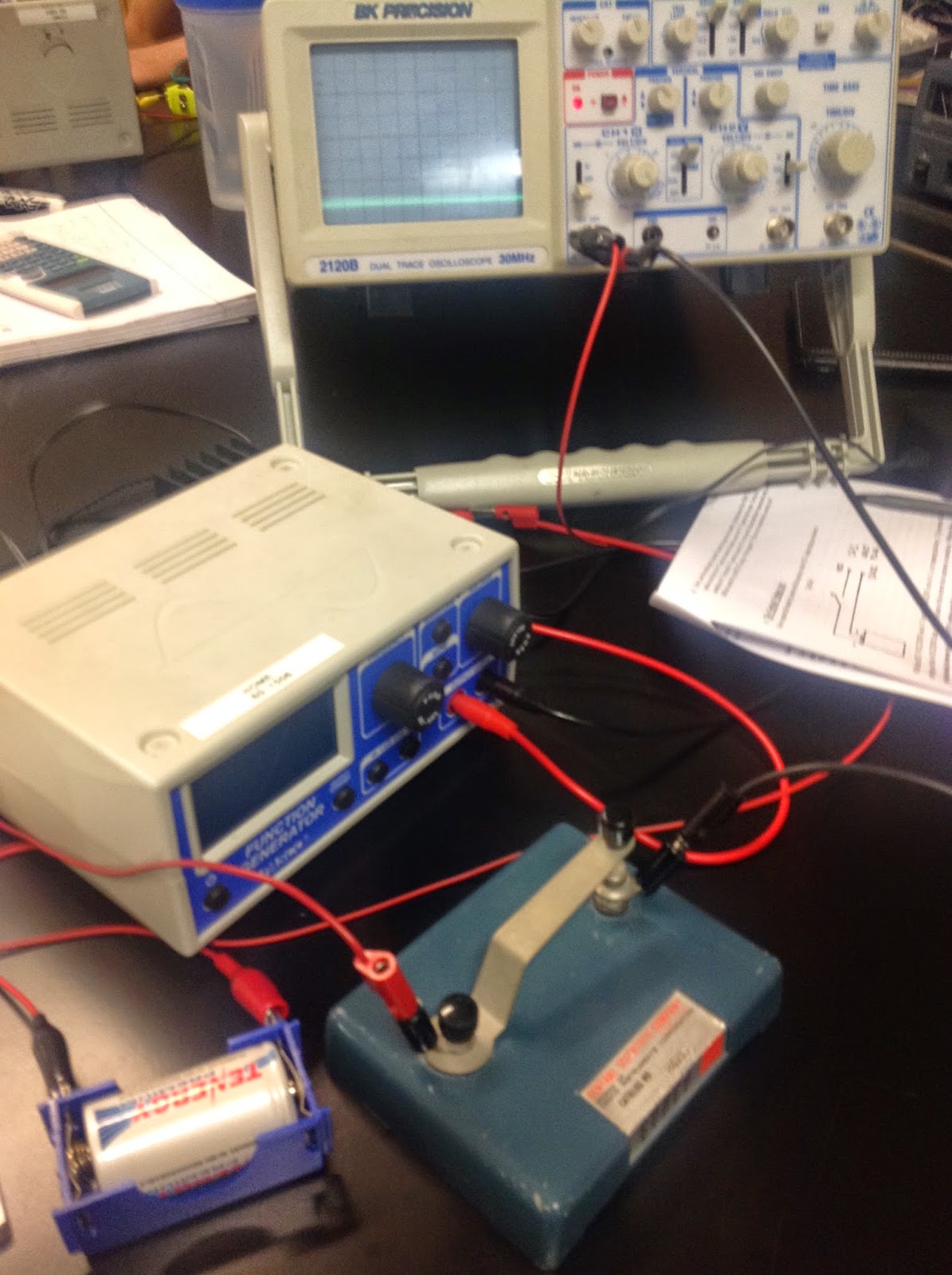

The next exercise consisted of measuring the voltage of two different power supplies and then using those measurements to compare the quality of each supply. We started off by measuring the voltage of a small table top power supply and found that there was a very fine amount of AC voltage that was delivered in the DC power supply's voltage. The next power supply measured was the output of a standard wall adapter. It was found that the voltage of the adapter varied greatly over time. It was concluded that the quality of the wall adapter was not very good.

After testing the power supplies, we moved on to an exercise involving Lissajous Figures. Pressing in the x-y button on the oscilloscope caused the display to enter a mode where channel 1 would drive the x-axis and channel 2 would drive the y-axis. Connecting function generators to both channels and setting both generators to varying frequencies cause the display to show various figures and shapes referred to as Lissajous Figures.


The final exercise of the day dealt with taking measurements from a box made up of unknown circuitry. Measurements showed that the box's circuits generated a variety of square wave functions.

The square waves generated by the box differed in duty cycle.

We started the day off with an kinematics exercise that had us find the distance an electron will travel between a set of charged plates. This exercise led to a live demonstration of an electron beam whose position was being aimed with external voltages on a series of plates that the beam traveled through. The purpose of this demonstration was to show the class the inner mechanics of the oscilloscopes display screen.
The next exercise of the day consisted of connecting a function generator to a speaker and having the generator output frequencies in the audible range. A function generator is a device that is capable of outputting an AC voltage at specific frequencies and wave shape. We learned that the frequency of the signal controls the pitch of the sound from the speaker, and the magnitude of the output voltage controlled the loudness.
The next exercise was measuring the voltage of a battery with the oscilloscope using a tap key in series with the battery. With the oscilloscope set to DC coupling, and appropriate values for volts/div and time/div set, we were able to measure the voltage of the battery at around 1.2 volts.
The next exercise consisted of measuring the voltage of two different power supplies and then using those measurements to compare the quality of each supply. We started off by measuring the voltage of a small table top power supply and found that there was a very fine amount of AC voltage that was delivered in the DC power supply's voltage. The next power supply measured was the output of a standard wall adapter. It was found that the voltage of the adapter varied greatly over time. It was concluded that the quality of the wall adapter was not very good.
After testing the power supplies, we moved on to an exercise involving Lissajous Figures. Pressing in the x-y button on the oscilloscope caused the display to enter a mode where channel 1 would drive the x-axis and channel 2 would drive the y-axis. Connecting function generators to both channels and setting both generators to varying frequencies cause the display to show various figures and shapes referred to as Lissajous Figures.
The final exercise of the day dealt with taking measurements from a box made up of unknown circuitry. Measurements showed that the box's circuits generated a variety of square wave functions.
The square waves generated by the box differed in duty cycle.
Mon. Week 10, April 28: The RC Time Constant
Today, the class went into depth on the span of time it takes for a capacitor to reach full charge. Capacitors do not come to full charge immediately after being connected to a voltage source. The time it takes to reach full charge and the factors that affect this time is all encompassed in the subject of RC time constants.
The first experiment of class dealt with generating a graph of voltage across the capacitor vs. time so we could then attempt to generate an equation for the time it takes for a capacitor to reach full charge. Logger pro was used to measure voltage over a span of time.

After a graph for the voltage vs. time for a charging capacitor was generated, it could be easily seen that the voltage followed a pattern of exponential growth. A line was fit to the curve and an exponential equation was generated.

We then made a new graph for the voltage vs. time of a capacitor while it was discharging. We observed a similar pattern to that of the charging graph.

After generating equations for the two graphs, we then sought out to try and make sense of the constants that were given by the generated equations. We determined that the constant A was simply the initial voltage that was recorded at the start of the data collection. Constant B was simply a very low value that could be interpreted as zero and having no influence on the final voltage. In order to solver the constant C, we had to find a way in which the time unit canceled out since the total equation was supposed to be only in units of voltage. Through some tricky algebra, we discovered that the value for C was 1/RC.

We learned that the value of RC is referred to as the RC time constant and is denoted by the Greek letter Tau. We then began to explore the properties of the time constant.

Soon, we predicted the graph of current vs. time while a capacitor was charging and then learned that current in an RC circuit could also be written as a function of the time constant Tau.

With knowledge of the time constant, we then preformed a series of problems that dealt with finding how long it would take for an capacitor to charge or discharge to a specific value.

The first experiment of class dealt with generating a graph of voltage across the capacitor vs. time so we could then attempt to generate an equation for the time it takes for a capacitor to reach full charge. Logger pro was used to measure voltage over a span of time.
After a graph for the voltage vs. time for a charging capacitor was generated, it could be easily seen that the voltage followed a pattern of exponential growth. A line was fit to the curve and an exponential equation was generated.
We then made a new graph for the voltage vs. time of a capacitor while it was discharging. We observed a similar pattern to that of the charging graph.
After generating equations for the two graphs, we then sought out to try and make sense of the constants that were given by the generated equations. We determined that the constant A was simply the initial voltage that was recorded at the start of the data collection. Constant B was simply a very low value that could be interpreted as zero and having no influence on the final voltage. In order to solver the constant C, we had to find a way in which the time unit canceled out since the total equation was supposed to be only in units of voltage. Through some tricky algebra, we discovered that the value for C was 1/RC.
We learned that the value of RC is referred to as the RC time constant and is denoted by the Greek letter Tau. We then began to explore the properties of the time constant.
Soon, we predicted the graph of current vs. time while a capacitor was charging and then learned that current in an RC circuit could also be written as a function of the time constant Tau.
With knowledge of the time constant, we then preformed a series of problems that dealt with finding how long it would take for an capacitor to charge or discharge to a specific value.
Mon. Week 9, April 21: Capacitance
This day's main topic of discussion was on the subject of capacitance, and the capacitor. The simple definition of capacitance is the potential difference between two conductors separated by an insulator. The charge on each conductor is opposite in polarity and the two charges remain stationary since they are attracted to each other through the insulator via their electric fields. The official definition of capacitance is the ratio of charge on each conductor and the potential difference across them.
The first exercise of the day was a derivation of the definition of capacitance as a function of the conductors' surface area and length of separation. It was found that capacitance is directly proportional to the surface area of the conductors and inversely proportional to the amount of distance between each conductor.

We then started an experiment to verify this proportionality of capacitance and surface area/distance. The experiment consisted of taking two sheets of conductive material (aluminum foil) and using a multimeter to measure the capacitance of the two sheets as the distance between them was increased and the surface area was decreased.

The gathered data verified the results predicted from the derivation we made at the start of class. As distance increased, the capacitance decreased, and as surface area decreased, the capacitance decreased.

The next segment of class was an introduction to the capacitor. The capacitor is a circuit component that is capable of storing energy in the form of an electric field.
One of the most important concepts to know on the topic of capacitors is equivalent capacitance. Much like resistors, the capacitance of a variety of capacitors in a circuit can be replaced by an equivalent capacitance based on whether the capacitors are hooked up in series or a parallel configuration.

We learned that capacitors in parallel are summed up, while capacitors in series are summed inversely, the opposite of combining resistors. We verified this by measuring the capacitance of capacitors in parallel and series.

The first exercise of the day was a derivation of the definition of capacitance as a function of the conductors' surface area and length of separation. It was found that capacitance is directly proportional to the surface area of the conductors and inversely proportional to the amount of distance between each conductor.
We then started an experiment to verify this proportionality of capacitance and surface area/distance. The experiment consisted of taking two sheets of conductive material (aluminum foil) and using a multimeter to measure the capacitance of the two sheets as the distance between them was increased and the surface area was decreased.
The gathered data verified the results predicted from the derivation we made at the start of class. As distance increased, the capacitance decreased, and as surface area decreased, the capacitance decreased.
The next segment of class was an introduction to the capacitor. The capacitor is a circuit component that is capable of storing energy in the form of an electric field.
One of the most important concepts to know on the topic of capacitors is equivalent capacitance. Much like resistors, the capacitance of a variety of capacitors in a circuit can be replaced by an equivalent capacitance based on whether the capacitors are hooked up in series or a parallel configuration.
We learned that capacitors in parallel are summed up, while capacitors in series are summed inversely, the opposite of combining resistors. We verified this by measuring the capacitance of capacitors in parallel and series.
Monday, April 21, 2014
Wed. Week 8, April 16: Resistors and Circuit analysis
On this day, the class went into further detail of electric circuits by focusing on the subject of circuit analysis. Particularly, we spent a large portion of time discussing the various ways in which a number of resistors could be connected together and how the various combination of ways to connect resistors can affect the overall resistance of the total circuit.
At the start of class, we were tasked with repeating the steps we took in the previous quiz where we had to connect two bulbs in a way to get either both bulbs dim or both bright.
After this was accomplished, we treated the bulbs as resistors and started taking voltage readings at points on both circuit configurations. We then solved for current at these points in both circuits. The values were then compared and a pattern was discovered regarding the configuration in which the bulbs were hooked up the the circuit.

This observation led to a discussion on equivalent resistance of resistors in parallel and series. The overall resistance of resistors in series is simply the summed up resistances of each resistor and the overall resistance of resistors in parallel are summed inversely.
With this knowledge, circuits made up of parallel and series combinations could now be reduced to a simpler circuit made up of equivalent resistances.
To demonstrate this property of resistors, the class first calculated the equivalent resistance of a given parallel-series circuit and then compared that value to the measured resistance of the built circuit. The two resistances proved to be equal to each other within the range of the resistors' tolerances.

At the start of class, we were tasked with repeating the steps we took in the previous quiz where we had to connect two bulbs in a way to get either both bulbs dim or both bright.
After this was accomplished, we treated the bulbs as resistors and started taking voltage readings at points on both circuit configurations. We then solved for current at these points in both circuits. The values were then compared and a pattern was discovered regarding the configuration in which the bulbs were hooked up the the circuit.
This observation led to a discussion on equivalent resistance of resistors in parallel and series. The overall resistance of resistors in series is simply the summed up resistances of each resistor and the overall resistance of resistors in parallel are summed inversely.
With this knowledge, circuits made up of parallel and series combinations could now be reduced to a simpler circuit made up of equivalent resistances.
To demonstrate this property of resistors, the class first calculated the equivalent resistance of a given parallel-series circuit and then compared that value to the measured resistance of the built circuit. The two resistances proved to be equal to each other within the range of the resistors' tolerances.
Tuesday, April 15, 2014
Mon. Week 8, April 14: Electric Potential
Today's topic of discussion was primarily focused on the subject of electric potential. Different from electric potential energy, electric potential is another word for describing voltage and is defined as potential energy per unit charge.
At the start of the class, we were given an exercise where we calculated the potential between each of twenty evenly distributed segments of an symmetrical geometric object at some point from the object.
The next major experiment dealt with taking live measurements of potential at different points between two points across a conductive sheet of paper. Fifteen volts was applied to the two strips of metallic paint shown on the paper. We measured voltage at points between the paint with respect to the round blotch of paint (not the long strip).

The data gathered from the potential measurements suggests that the potential increases non-linearly


At the start of the class, we were given an exercise where we calculated the potential between each of twenty evenly distributed segments of an symmetrical geometric object at some point from the object.
The next major experiment dealt with taking live measurements of potential at different points between two points across a conductive sheet of paper. Fifteen volts was applied to the two strips of metallic paint shown on the paper. We measured voltage at points between the paint with respect to the round blotch of paint (not the long strip).
The data gathered from the potential measurements suggests that the potential increases non-linearly
Wed. Week 7, April 9: More with circuits
For this day, we went more into depth on the topic of electric circuits and their properties.
At the beginning of class, we started with a quiz that tasked us in developing a way of wiring a series of two light bulbs in a configuration where one light would be dim, or both would be bright. The secret to success on this quiz is being familiar with the properties of series and parallel circuits. The bulbs wired up in a parallel to the voltage source would both be bright since the voltage down each branch would be the same as the voltage at the source. The bulbs wired in series with the voltage source would produce a bright and a dim bulb since there is a voltage drop across the first bulb, causing the second bulb to be powered with lesser voltage.

We then viewed a demonstration on the relationship of power and heat. The cup was filled with a saline solution that was used as a conductor between two electrodes. Voltage was applied to the electrodes and a temperature probe measured any increase in temperature of the solution.

From the graph generated by the temperature data, we could solve for values such as resistance and current. The sharp jump in the graph corresponds to an increase of the voltage settings.

Toward the end of class, we watched another demonstration regarding the generating of heat using the internal resistance of food products as a circuit's load. With a high enough voltage, the power through the hot dog was enough to char the ends where the electrodes were attached and cause some mild smoking. Another experiment was performed from the hot dog set up, which dealt with the how the spacing of LED leads would contribute to the power generated by them. It turns out that the LED that was stuck into the hot dog resistor with the largest lead gap was the one that generated the most power. This observation was due to the fact that the wider lead spacing directly related to a larger potential difference across those leads.

At the beginning of class, we started with a quiz that tasked us in developing a way of wiring a series of two light bulbs in a configuration where one light would be dim, or both would be bright. The secret to success on this quiz is being familiar with the properties of series and parallel circuits. The bulbs wired up in a parallel to the voltage source would both be bright since the voltage down each branch would be the same as the voltage at the source. The bulbs wired in series with the voltage source would produce a bright and a dim bulb since there is a voltage drop across the first bulb, causing the second bulb to be powered with lesser voltage.
We then viewed a demonstration on the relationship of power and heat. The cup was filled with a saline solution that was used as a conductor between two electrodes. Voltage was applied to the electrodes and a temperature probe measured any increase in temperature of the solution.
From the graph generated by the temperature data, we could solve for values such as resistance and current. The sharp jump in the graph corresponds to an increase of the voltage settings.
Toward the end of class, we watched another demonstration regarding the generating of heat using the internal resistance of food products as a circuit's load. With a high enough voltage, the power through the hot dog was enough to char the ends where the electrodes were attached and cause some mild smoking. Another experiment was performed from the hot dog set up, which dealt with the how the spacing of LED leads would contribute to the power generated by them. It turns out that the LED that was stuck into the hot dog resistor with the largest lead gap was the one that generated the most power. This observation was due to the fact that the wider lead spacing directly related to a larger potential difference across those leads.
Subscribe to:
Posts (Atom)